Using cosmological surveys to map out the invisible (and the visible) matter
Yuuki Omori (U.Chicago/KICP)
Credit: Aman Chokshi (2021 Winter Over)


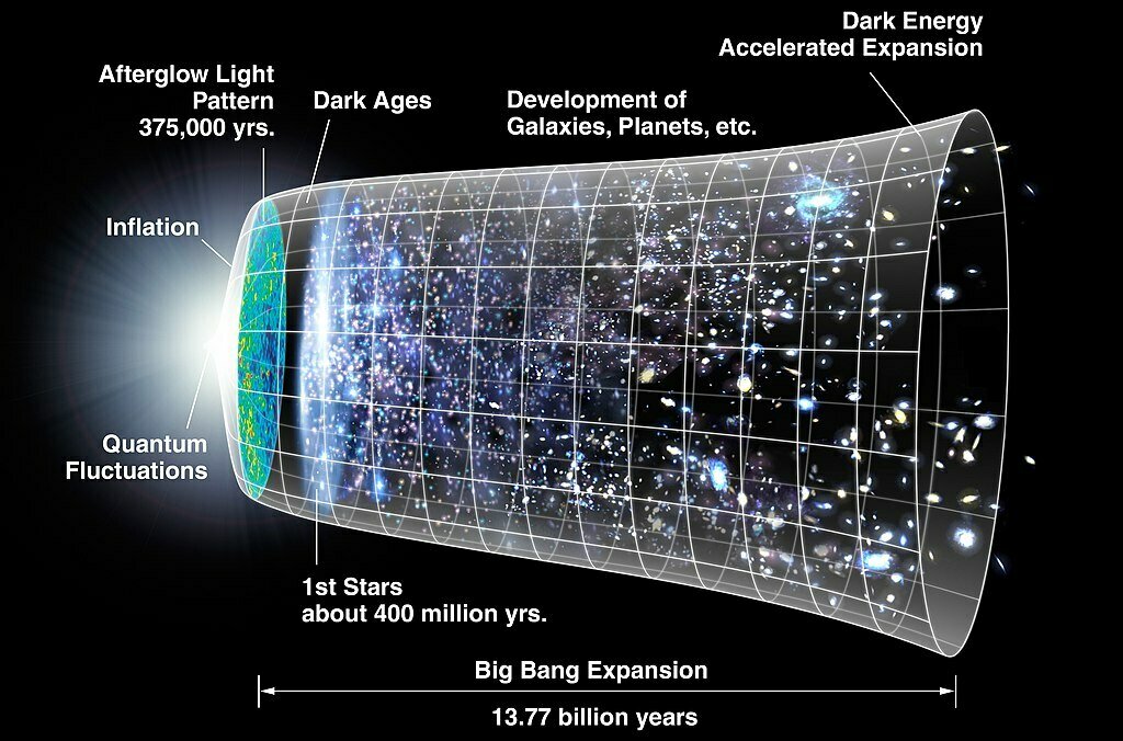
Cosmic history
1
Cosmic microwave background
Cosmology
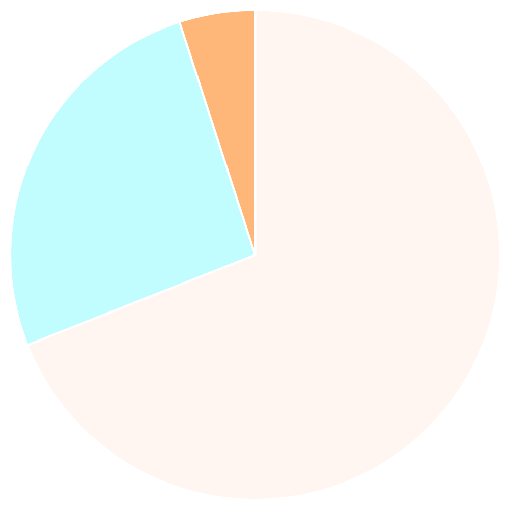
Dark energy
Dark matter
Ordinary matter
(5%)
(26%)
(69%)
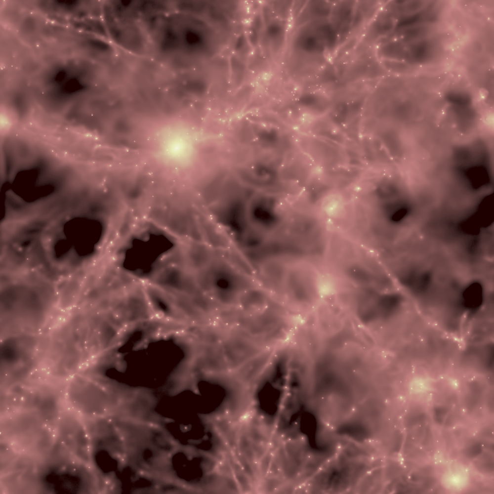
The goal of this talk is to describe how we map the distribution of invisible and visible matter
2
Weak gravitational lensing
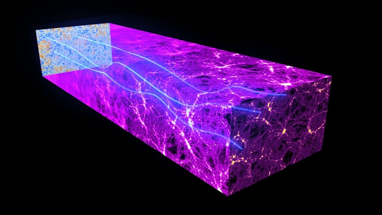
Background light
Matter between
the light source and us
3
Weak gravitational lensing
Cosmic microwave background
(Undistored temperature map)
Cosmic microwave background
(Distorted temperature map)
4
Distant galaxies
Nearby massive
object
Undistorted background
galaxy image
Cosmic microwave background
(Undistored temperature map)
Cosmic microwave background
(Distorted temperature map)
4
Weak gravitational lensing
Nearby massive
object
Distorted background
galaxy image
Cosmic microwave background
(Undistored temperature map)
Cosmic microwave background
(Distorted temperature map)
4
Weak gravitational lensing
Distant galaxies
Reconstruction approach
CMB lensing
3D gravitational potential
5
Reconstruction approach
CMB lensing
3D gravitational potential
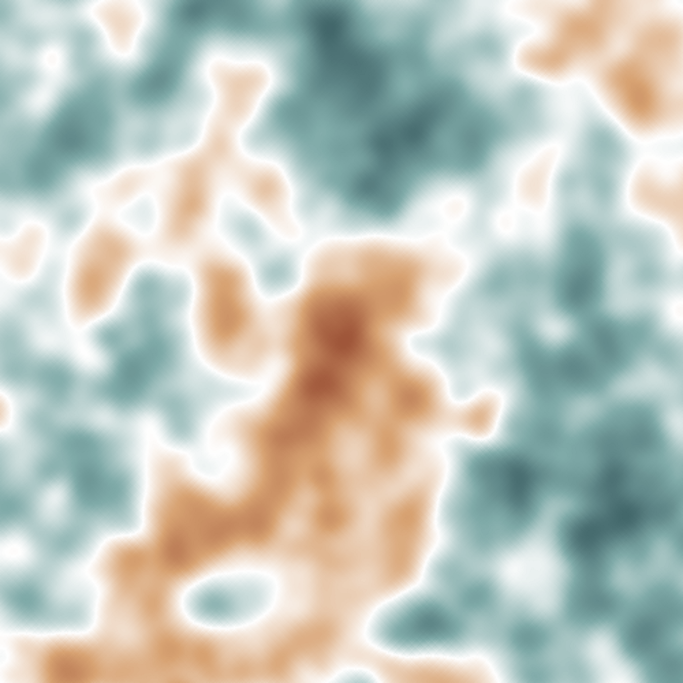
2D potential
5
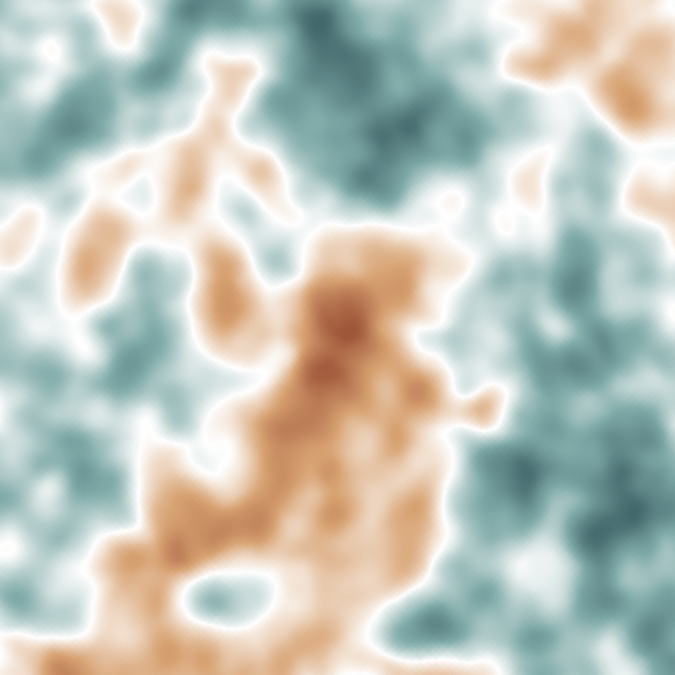
Reconstruction approach
CMB lensing
3D gravitational potential
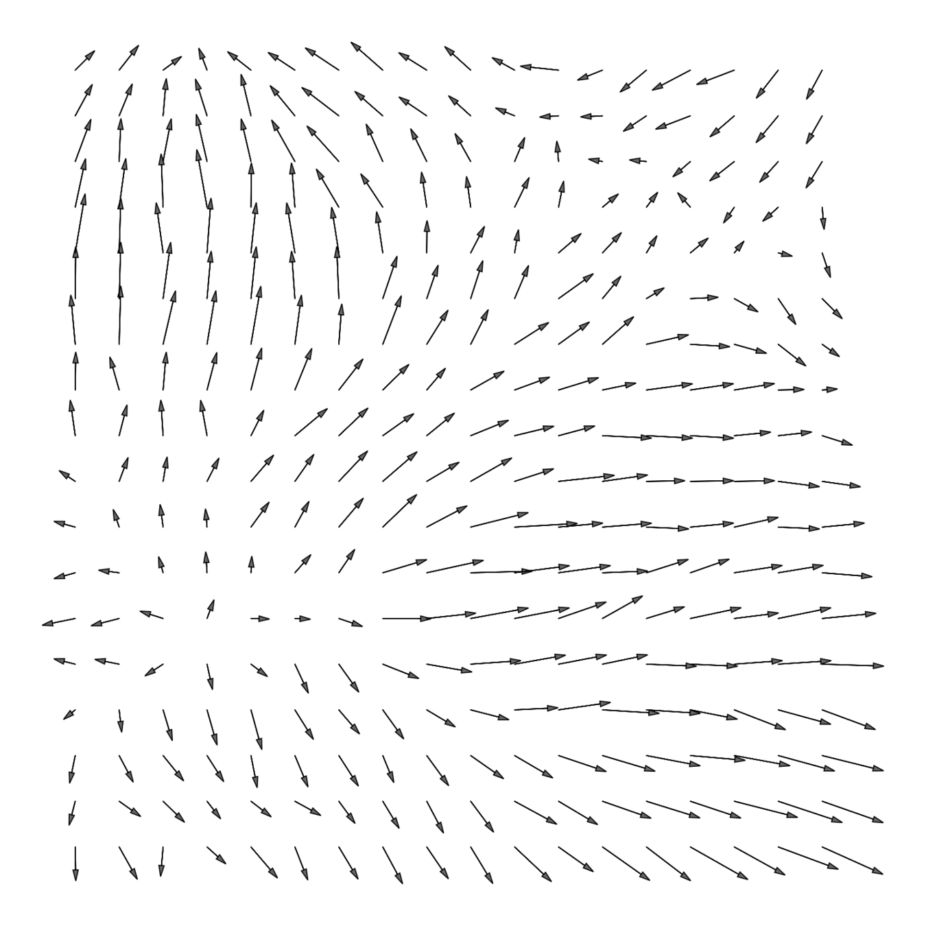
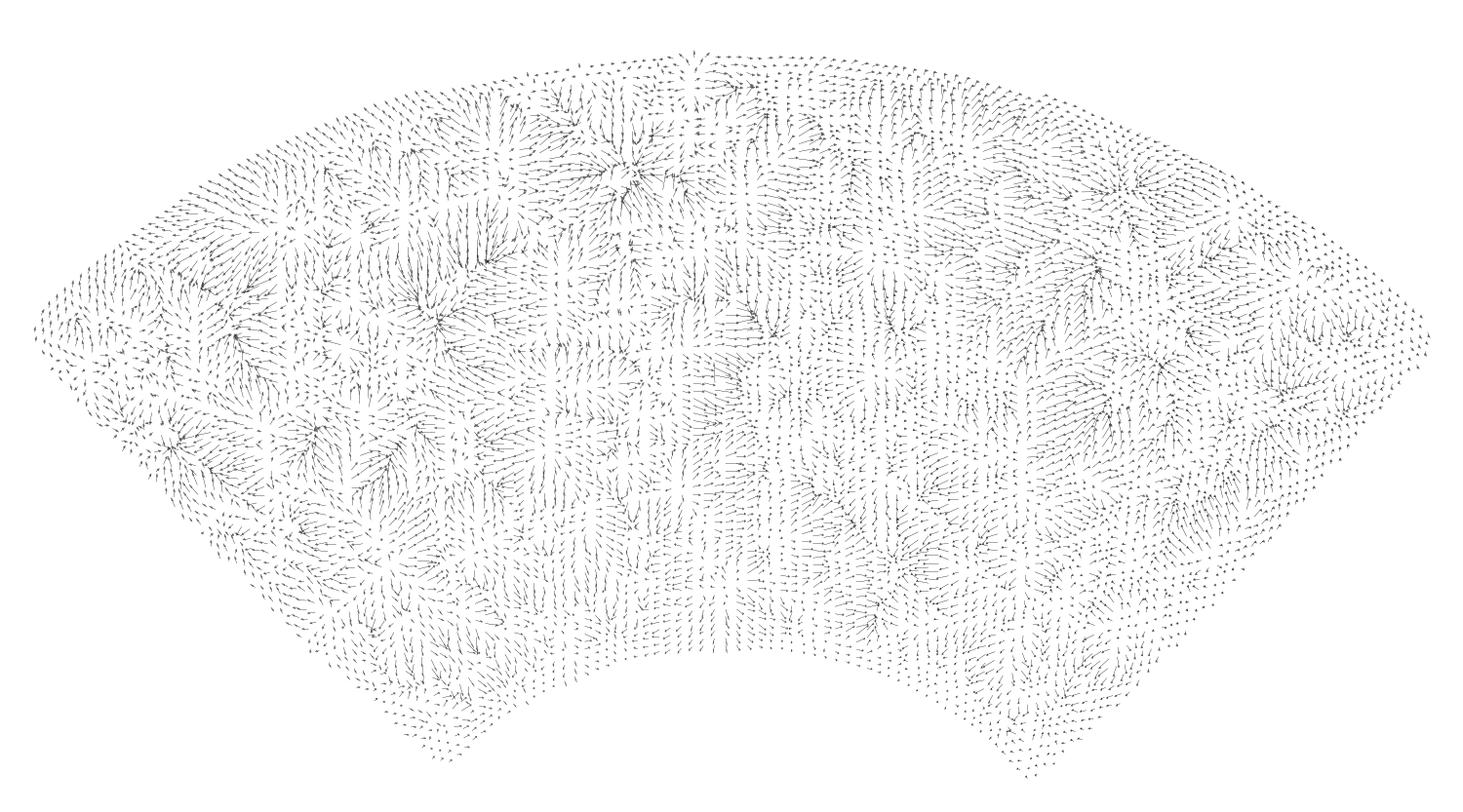
2D potential
Deflection
5
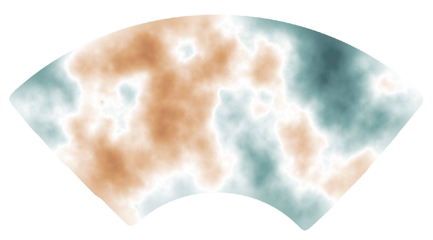
Convergence
Reconstruction approach
CMB lensing
Two independent modes become correlated through the lensing potential
6
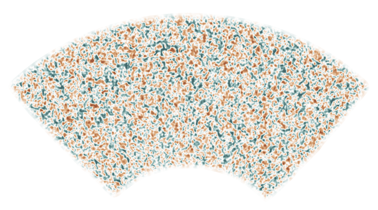
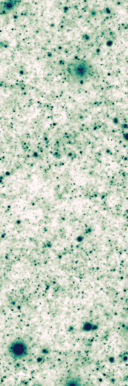
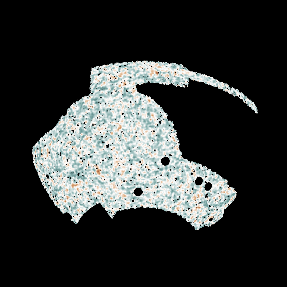
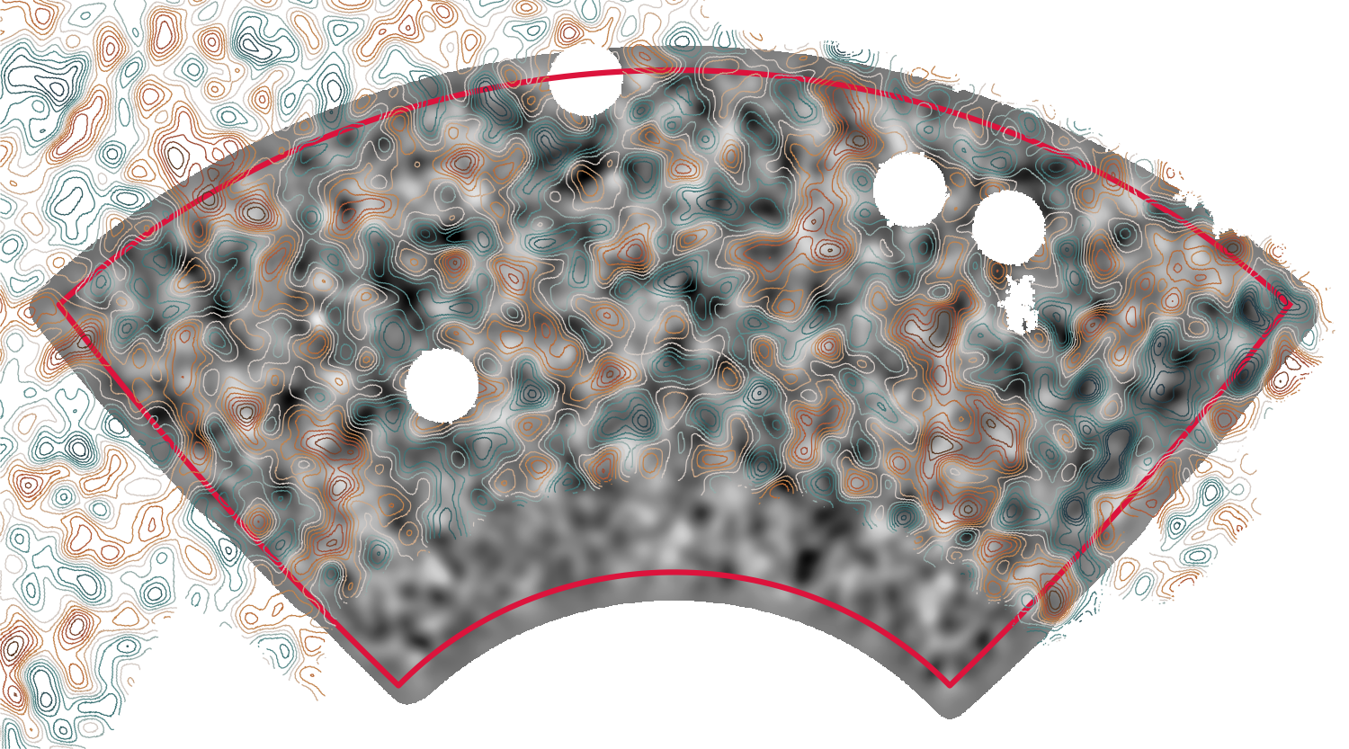
SPT-3G lensing map
(see also: Omori2017, Omori2023)
7
Reconstruction approach
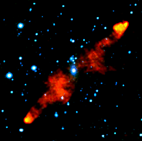
CMB lensing - challenges (foregrounds)
8
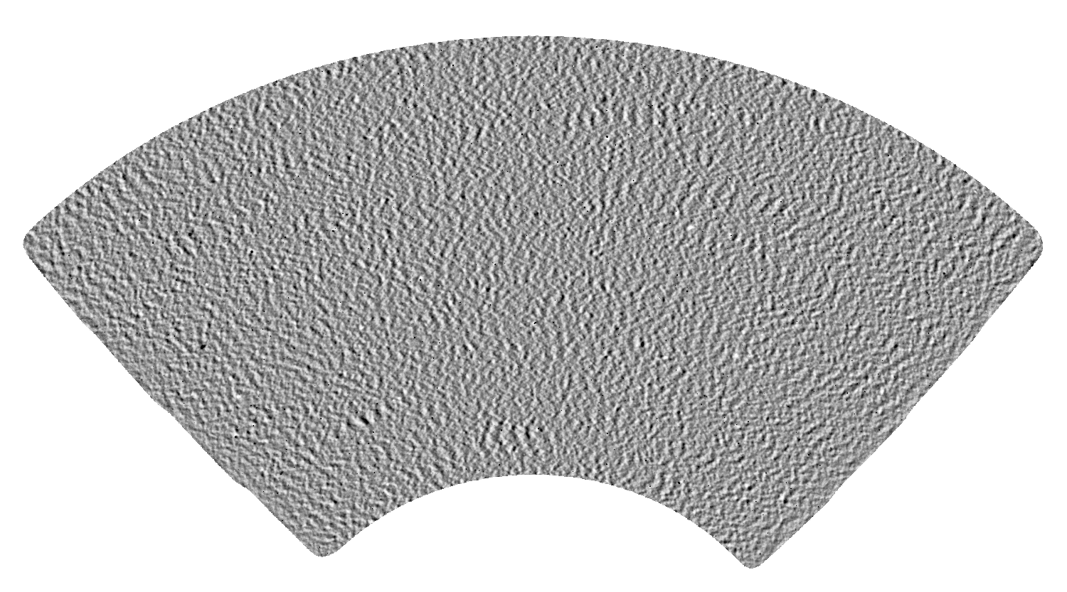
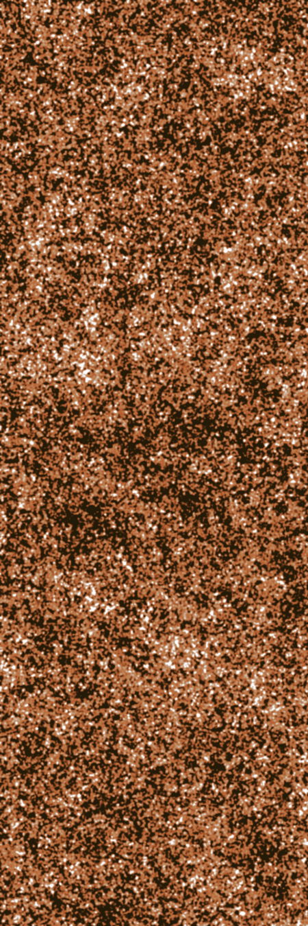
SPT-3G temperature map
Reconstruction approach
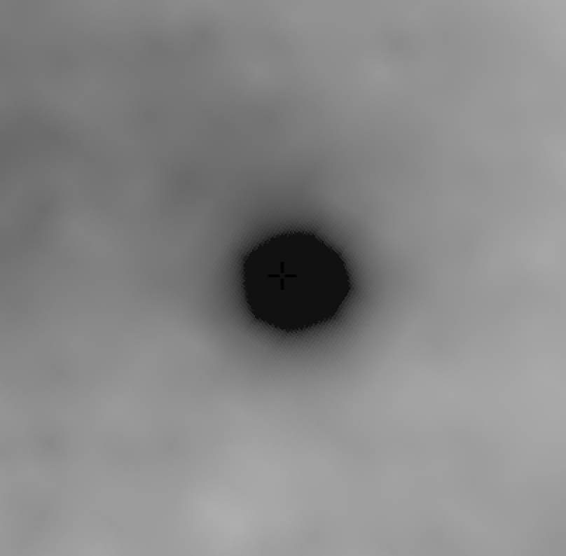
CMB lensing - challenges (foregrounds)
SPT-3G temperature map
SPT-CLJ0234-5831
8
Reconstruction approach
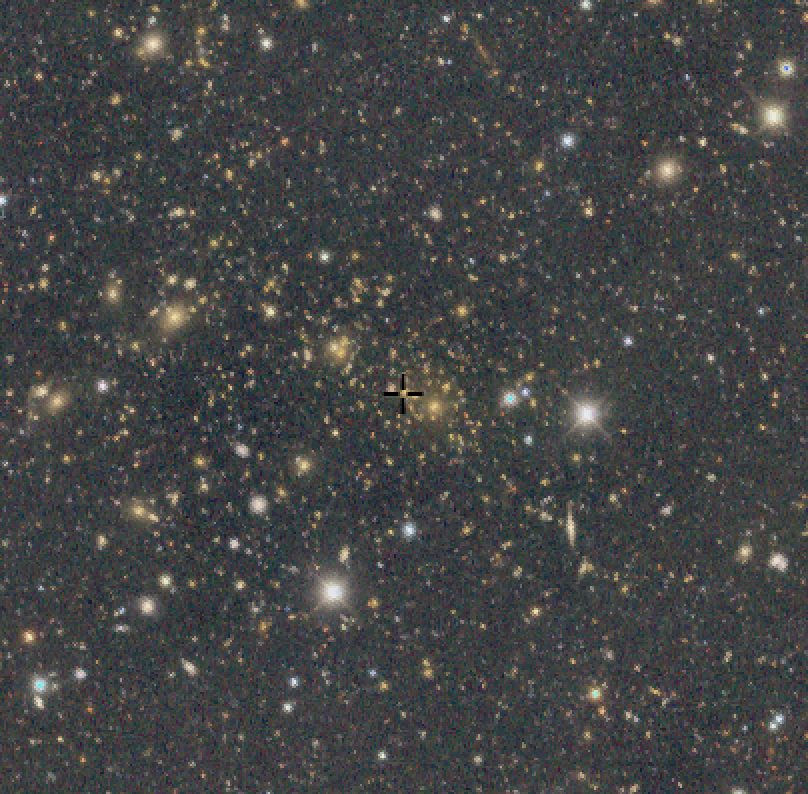
CMB lensing - challenges (foregrounds)
SPT-3G temperature map
SPT-CLJ0234-5831
8
Reconstruction approach
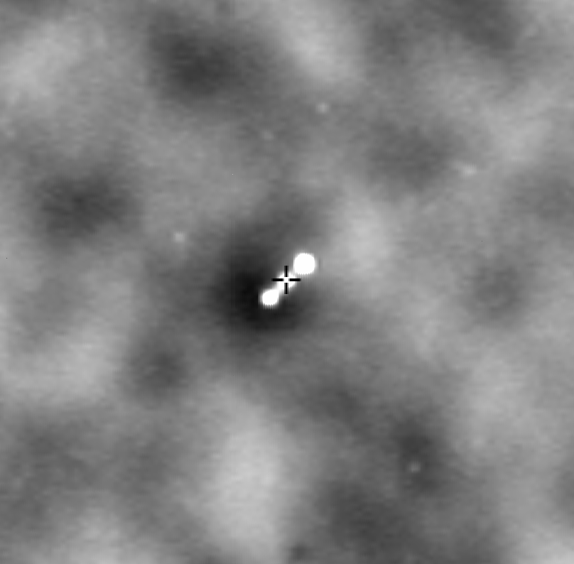
CMB lensing - challenges (foregrounds)
SPT-3G temperature map
PKS 2356-61
SPT-CLJ0234-5831
8
Reconstruction approach
CMB lensing - challenges (foregrounds)
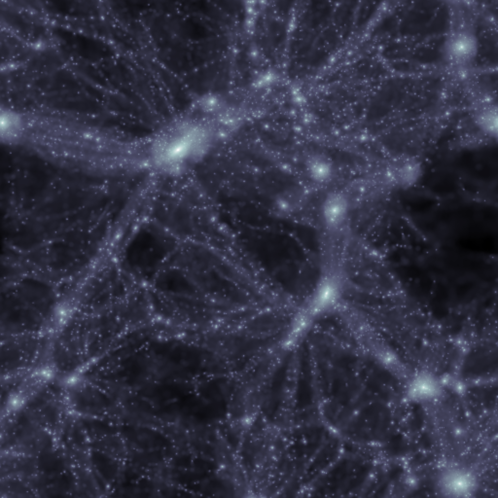
Agora simulation (Omori 2022)
Multi-Dark Planck 2
N-body simulation
(Klypin et al. 2017)

9
tSZ
kSZ
CIB
radio
Reconstruction approach
Galaxy lensing
10
(see Tianao & Emma's paper)
Reconstruction approach
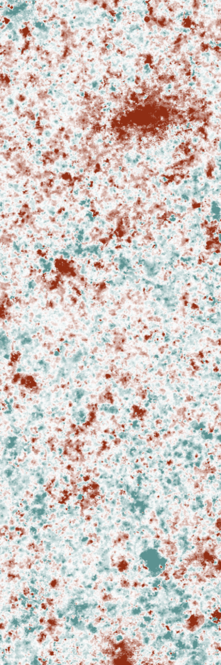
Galaxy lensing map
11
Jeffery2021
Map of from the
Dark Energy Survey
Reconstruction approach
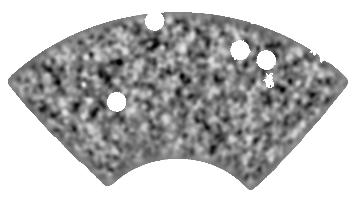
DES galaxy lensing
map (overlay)
SPT-3G CMB lensing map (base)
Lensing map comparison
12
(see also: Omori2018, Chang2023)
Forward modeling approach
Increasing number people have started to work on forward modeling approach due to increased computational power.
Gravitational/hydro-dynamical simulation
Ray-tracing
(light-propagation)
Predicted observed fields
Comparison with data
Computationally expensive
Repeat until predicted maps look like data
Approximate methods
13
Forward modeling approach
15
Preliminary work
Galaxy lensing forward modeling (fixed seed)
Forward modeling approach
Galaxy lensing forward modeling (varying seed)
16
Preliminary work
(Millea et al. 2021)
CMB lensing forward modeling
Forward modeling approach
14
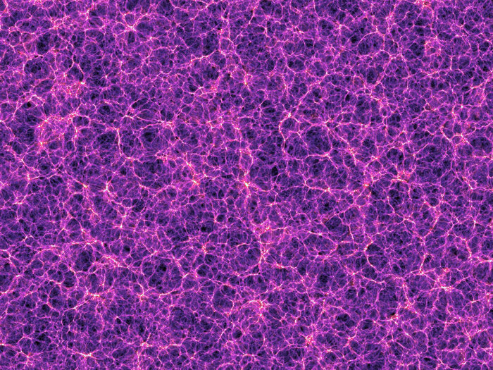
Total matter
Dark energy
Dark matter
Ordinary matter
(5%)
(26%)
(69%)
17
Forward modeling approach
Challenges (Impact of astrophysical effects)
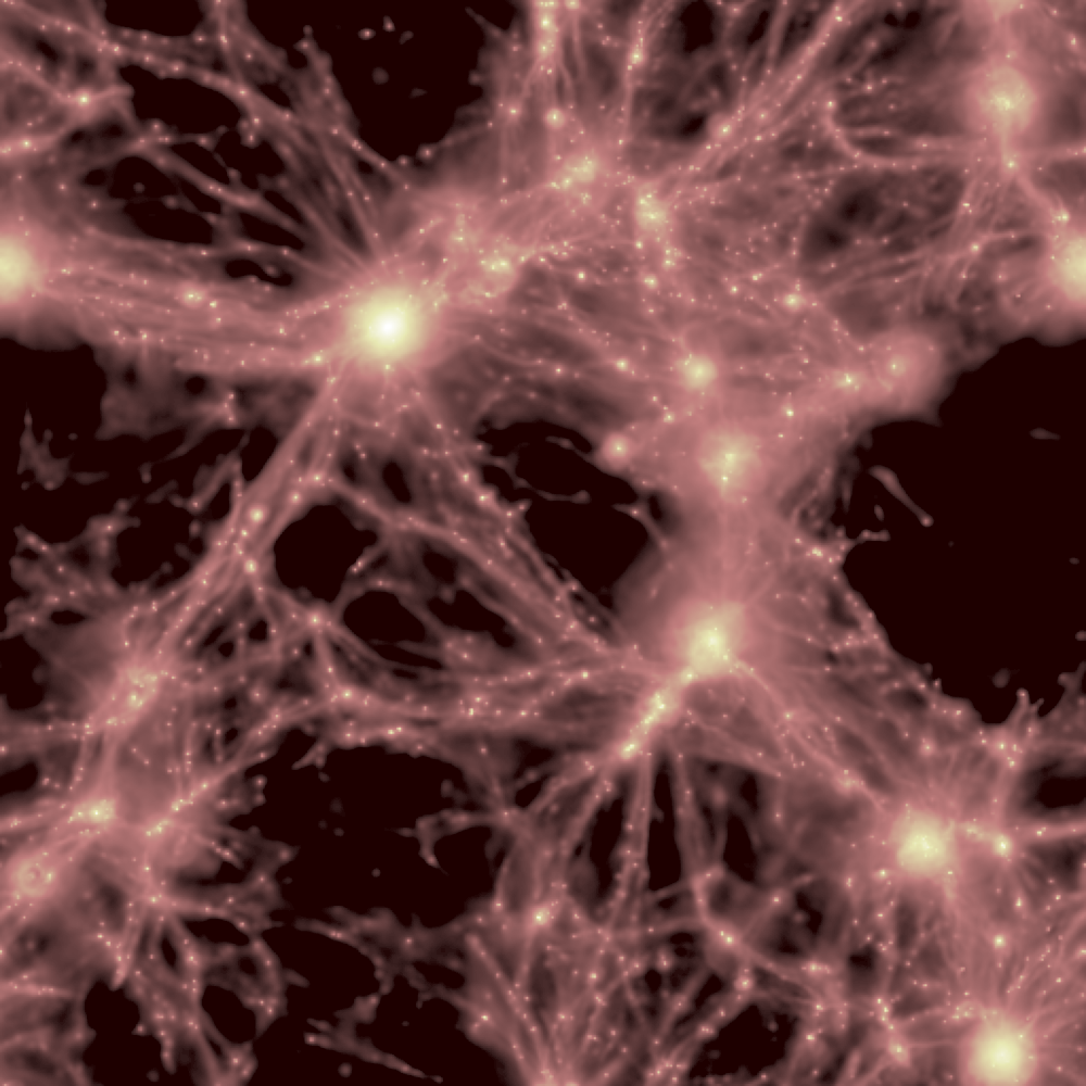
Dark matter
Ordinary matter (gas/stars)
18
Forward modeling approach
Challenges (Impact of astrophysical effects)
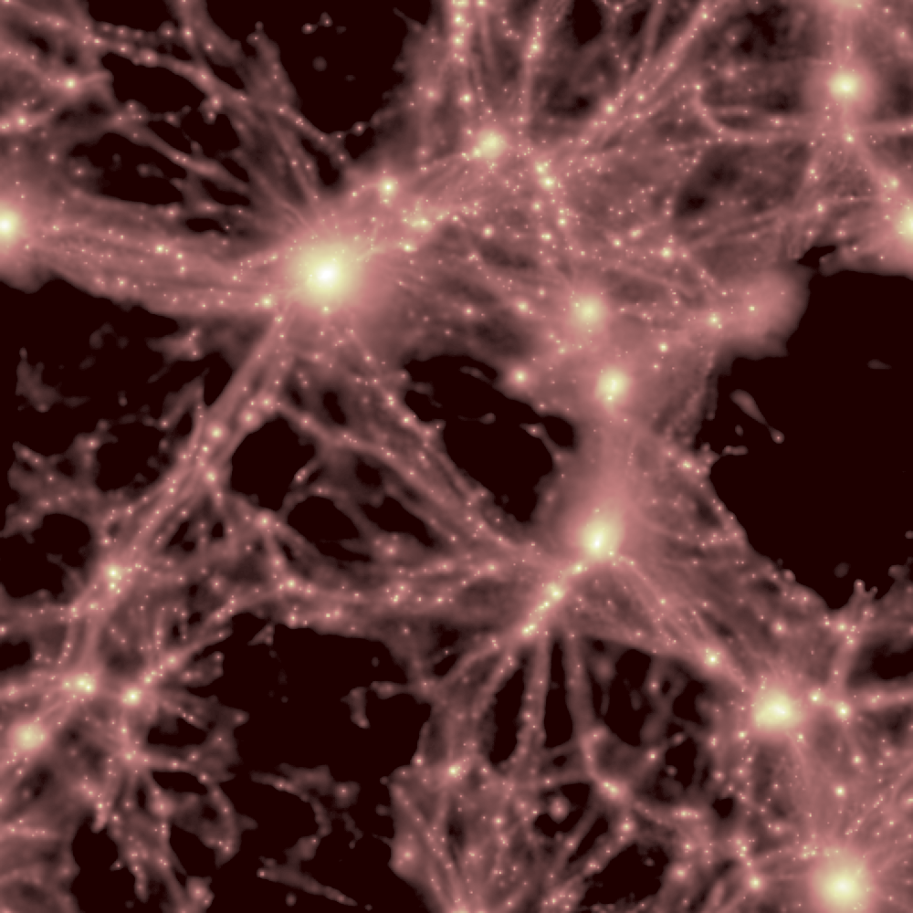
Illustris
Astrid
Simba
19
Forward modeling approach
Challenges (Impact of astrophysical effects)
Incoming data
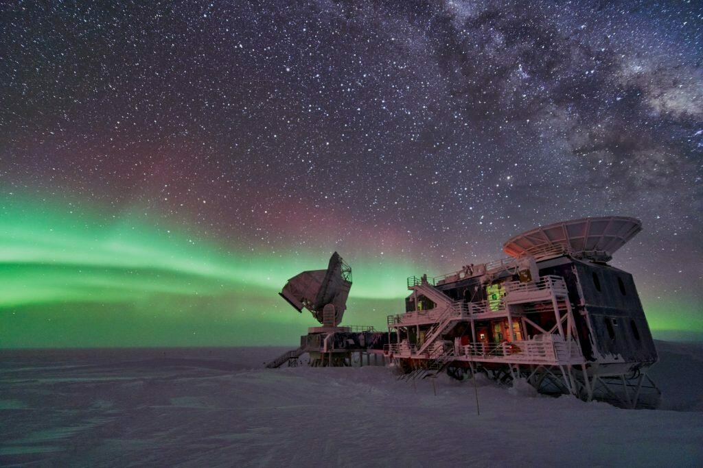
Simons Observatory/CMB-S4
South Pole Observatory/CMB-S4
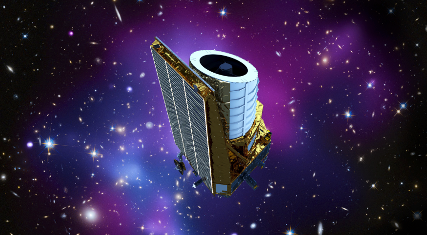
Euclid
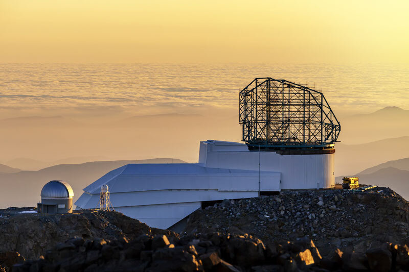
Rubin/LSST
20
Summary
21
- A map of the total matter distribution can be made using the weak gravitational lensing effect.
- Two different types of backlight can be used: cosmic microwave background and distant galaxies.
- Both approaches have their own challenges.
- Forward modeling approaches are starting to gain more attention due to increased computational capabilities and efficiency.
- Currently at an exciting time -- we already have good data, but the quality will become orders of magnitude better soon.